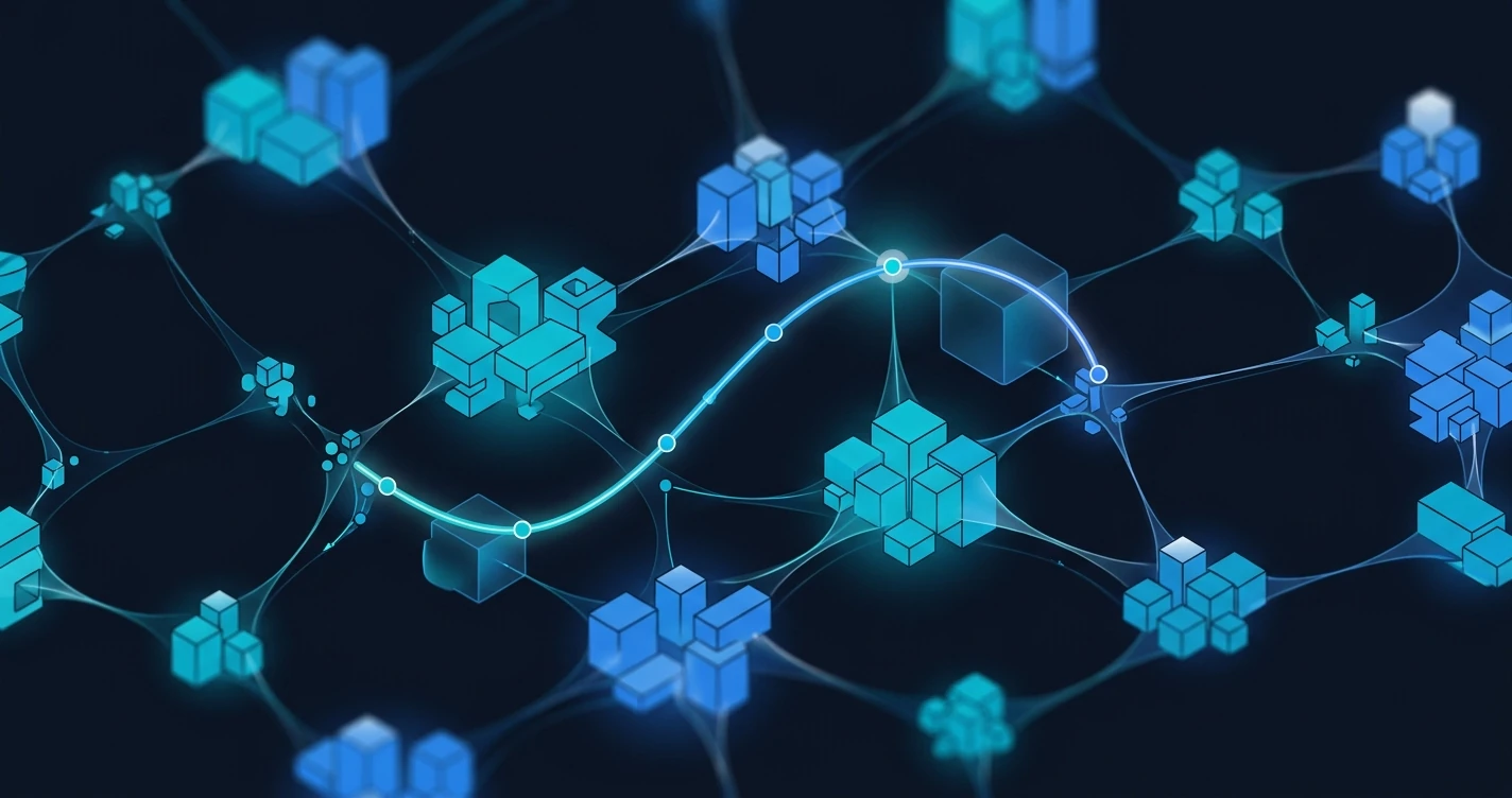
Navigating the latent space

Every image you've ever seen, every sentence you've read, lives in a space of absurd dimensionality. A 256x256 RGB image is a point in 196,608-dimensional space. A 50,000-token vocabulary gives each word a one-hot vector with 50,000 dimensions. Working directly in those raw spaces is computationally brutal and, more to the point, semantically useless. Most of that space is empty. The interesting structure lives on a much smaller manifold, and finding that manifold is the whole game.

What is a latent space

A latent space is a compressed, learned representation of your data. Instead of describing an image pixel by pixel, the model learns to describe it with a compact vector — say 128 or 256 dimensions — that captures the factors that actually vary: pose, lighting, identity, style. The word "latent" is from statistics, meaning hidden or unobserved. These are the variables the model infers, not the ones you hand it.

If your data lives in a high-dimensional space X, a latent space Z is a lower-dimensional space such that a mapping f: X → Z preserves the structure that matters for your task. The encoder compresses, the decoder reconstructs. What sits between them is the latent space.

How autoencoders build them

The simplest architecture for learning a latent space is the autoencoder. Two networks: an encoder that maps input x to a latent vector z, and a decoder that maps z back to a reconstruction x'. Train it to minimize reconstruction loss — typically mean squared error for continuous data, binary cross-entropy for binary data.

import torch
import torch.nn as nn

class Autoencoder(nn.Module):
    def __init__(self, input_dim=784, latent_dim=32):
        super().__init__()
        self.encoder = nn.Sequential(
            nn.Linear(input_dim, 256),
            nn.ReLU(),
            nn.Linear(256, latent_dim)
        )
        self.decoder = nn.Sequential(
            nn.Linear(latent_dim, 256),
            nn.ReLU(),
            nn.Linear(256, input_dim),
            nn.Sigmoid()
        )

    def forward(self, x):
        z = self.encoder(x)
        return self.decoder(z)

The bottleneck forces compression. The vanilla autoencoder has one ugly issue, though: the latent space it produces is often irregular, with gaps and discontinuities. That makes sampling new points or interpolating smoothly hard.

Variational autoencoders smooth it out

The Variational Autoencoder (VAE), from Kingma and Welling in 2013, fixes this by imposing structure on the latent space. The encoder doesn't output a single point; it outputs the parameters of a probability distribution — specifically the mean and log-variance of a Gaussian. The model samples from that distribution during training, and a KL divergence term in the loss pushes those distributions toward a standard normal prior.

The loss combines reconstruction accuracy with a regularizer:

L = E[log p(x|z)] - KL(q(z|x) || p(z))

The result is a latent space that's continuous (nearby points decode to similar outputs) and complete (every point in the space decodes to something plausible). That's what makes VAEs generative: sample a random vector from the prior, decode it, get a realistic output.

Interpolation and arithmetic

One of the cool properties of a well-structured latent space: linear operations correspond to semantic operations. Encode two images — a face with glasses and a face without — and interpolate between their latent vectors, decoding each intermediate point. You get a smooth morph between the two faces, glasses gradually appearing or disappearing.

Latent arithmetic is even more striking. The famous word2vec example applies: take the vector for "man with glasses," subtract "man without glasses," add "woman without glasses," and you get something close to "woman with glasses." It works because the model has disentangled "wearing glasses" into a direction in latent space.

# Latent arithmetic example
z_glasses = encoder(man_with_glasses)
z_no_glasses = encoder(man_without_glasses)
z_woman = encoder(woman_without_glasses)

z_result = z_woman + (z_glasses - z_no_glasses)
generated = decoder(z_result)  # woman with glasses

This isn't a trick. It reflects genuine structure in the learned representation. When the latent space disentangles factors of variation, each direction corresponds to a meaningful attribute.

What it actually powers

Latent spaces aren't just academically interesting. Real systems run on them.

Image generation. Stable Diffusion operates in the latent space of a pretrained autoencoder. Diffusing and denoising in pixel space would be computationally brutal; the process happens in a much smaller latent space, then the decoder maps back to pixels. That's what makes high-resolution image generation tractable.

Drug discovery. Molecules can be encoded into a continuous latent space where proximity matches structural and functional similarity. Researchers optimize in that space to find molecules with desired properties — latent space optimization. Far more efficient than searching the discrete space of molecular graphs.

Anomaly detection. Train an autoencoder on normal data and anomalous inputs will have high reconstruction error because they fall outside the learned manifold. The latent space gives you a compact feature space where distance-based anomaly detection just works.

Recommendation systems. Collaborative filtering models like matrix factorization are basically learning a shared latent space for users and items. A user's latent vector captures their preferences, an item's latent vector captures its attributes, and the dot product predicts affinity.

Exploring and debugging latent representations

When something goes wrong with a generative model, the latent space is the first place to look.

Dimensionality reduction. Apply t-SNE or UMAP to your latent vectors and color them by known labels. If your VAE is supposed to model digits, you should see ten distinct clusters. If classes overlap heavily, the model hasn't learned useful structure.

Interpolation tests. Pick two points and decode 10 intermediate steps. Smooth transitions mean the space is well-organized. Abrupt jumps or nonsense outputs mean there are holes in the manifold.

Traversal along axes. Fix all dimensions except one and vary it across its range. With disentangled representations, each dimension controls a single interpretable factor. If changing one dimension alters multiple attributes at once, the representation is entangled.

Posterior collapse. In VAEs, if the KL divergence term drops to near zero during training, the encoder has learned to ignore the input and always output the prior. The decoder then relies entirely on its own capacity. Common failure mode, usually fixed with KL annealing or a weaker decoder.

The manifold hypothesis

All of this rests on one assumption: real-world high-dimensional data doesn't fill its ambient space uniformly. It concentrates near a lower-dimensional manifold. A 64x64 face image has 12,288 dimensions, but the space of plausible faces is far smaller. The latent space is our best approximation of that manifold.

That's why latent spaces work. The data has structure, and the model exposes that structure in a form we can compute with. The better the model captures the true manifold, the more useful the latent space becomes for generation, interpolation, search, and understanding.

If you work with modern generative AI, you can't avoid latent spaces. Whether you're debugging a diffusion model, building a recommender, or trying to figure out why your VAE produces blurry images, the answer usually lives somewhere in the geometry of the latent space.